
N-grams Embeddings - Cosine Similarity Analysis
Contents
N-grams Embeddings - Cosine Similarity Analysis
Next, we look into cosine similarity distances to measure the descripiton similarity between companies. In this notebook, we simply use n-grams embeddings for consine similarity analysis.
Cosine similarity measures the similarity between two vectors of an inner product space. In text analysis, a document can be represented by its elements (words) and the frequency of each element. Comparing the frequency of words in different documents, which is the company description for companies in our case, would generate cosine similarity distance between documents. Each description generates a vector containing the frequency of each word. It measures the similarity between these companies in terms of their business description.
import pandas as pd
import numpy as np
import matplotlib.pyplot as plt
import seaborn as sns
df = pd.read_csv('../data/preprocessed.csv',
                usecols = ['reportingDate', 'name',
                           'coDescription_stopwords', 'SIC', 'SIC_desc'])
Cosine Similarity Analysis
Words Counting
For this cosine similarity analysis, we generate sequences of 2 to 4 words as one term and only select the top 600 terms by frequency.
from sklearn.feature_extraction.text import CountVectorizer

Vectorizer = CountVectorizer(ngram_range = (2,4),
                             max_features = 600)

count_data = Vectorizer.fit_transform(df['coDescription_stopwords'])
wordsCount = pd.DataFrame(count_data.toarray(),columns=Vectorizer.get_feature_names())
wordsCount = wordsCount.set_index(df['name'])
Here is the n-grams embedding matrix with the 600 2-to-4 grams as columns and the 675 companies as rows.
wordsCount
| ability make | accounting standard | acquire property | act act | act amended | additional information | adequately capitalized | adverse effect | adverse effect business | adverse event | ... | wa million | weighted average | well capitalized | wholly owned | wholly owned subsidiary | wide range | within day | working interest | year ended | year ended december | |
|---|---|---|---|---|---|---|---|---|---|---|---|---|---|---|---|---|---|---|---|---|---|
| name | |||||||||||||||||||||
| MONGODB, INC. | 0 | 0 | 0 | 0 | 0 | 0 | 0 | 0 | 0 | 0 | ... | 0 | 0 | 0 | 0 | 0 | 3 | 0 | 0 | 5 | 0 |
| SALESFORCE COM INC | 0 | 0 | 0 | 0 | 0 | 0 | 0 | 0 | 0 | 0 | ... | 0 | 0 | 0 | 0 | 0 | 0 | 0 | 0 | 0 | 0 |
| SPLUNK INC | 0 | 0 | 0 | 0 | 1 | 2 | 0 | 0 | 0 | 0 | ... | 0 | 0 | 0 | 0 | 0 | 0 | 0 | 0 | 0 | 0 |
| OKTA, INC. | 0 | 0 | 0 | 0 | 0 | 1 | 0 | 0 | 0 | 0 | ... | 0 | 0 | 0 | 0 | 0 | 1 | 0 | 0 | 1 | 0 |
| VEEVA SYSTEMS INC | 0 | 12 | 0 | 1 | 4 | 1 | 0 | 7 | 4 | 0 | ... | 18 | 4 | 0 | 0 | 0 | 0 | 1 | 0 | 102 | 0 |
| ... | ... | ... | ... | ... | ... | ... | ... | ... | ... | ... | ... | ... | ... | ... | ... | ... | ... | ... | ... | ... | ... |
| AMERICAN REALTY CAPITAL NEW YORK CITY REIT, INC. | 0 | 0 | 1 | 0 | 0 | 1 | 0 | 1 | 0 | 0 | ... | 0 | 0 | 0 | 0 | 0 | 0 | 0 | 0 | 2 | 2 |
| CYCLACEL PHARMACEUTICALS, INC. | 0 | 0 | 0 | 0 | 0 | 1 | 0 | 1 | 0 | 1 | ... | 0 | 0 | 0 | 0 | 0 | 0 | 1 | 0 | 0 | 0 |
| ZOETIS INC. | 0 | 17 | 0 | 0 | 0 | 12 | 0 | 3 | 0 | 0 | ... | 20 | 5 | 0 | 1 | 1 | 0 | 2 | 0 | 84 | 83 |
| STAG INDUSTRIAL, INC. | 0 | 0 | 1 | 0 | 1 | 0 | 0 | 1 | 1 | 0 | ... | 0 | 0 | 0 | 0 | 0 | 0 | 0 | 0 | 2 | 2 |
| EQUINIX INC | 0 | 0 | 0 | 0 | 2 | 0 | 0 | 0 | 0 | 0 | ... | 0 | 0 | 0 | 0 | 0 | 0 | 0 | 0 | 2 | 2 |
675 rows × 600 columns
Cosine Similarity Computation
Now we take in the 2-to-4 grams embeddings to analyze the text similarity.
# Compute Cosine Similarity
from sklearn.metrics.pairwise import cosine_similarity
cosine_sim = pd.DataFrame(cosine_similarity(wordsCount, wordsCount))
cosine_sim = cosine_sim.set_index(df['name'])
cosine_sim.columns = df['name']
The description similarity between companies range from 0 to 1. The higher the cosine similarity score, the more similar they are.
cosine_sim
| name | MONGODB, INC. | SALESFORCE COM INC | SPLUNK INC | OKTA, INC. | VEEVA SYSTEMS INC | AUTODESK INC | INTERNATIONAL WESTERN PETROLEUM, INC. | DAYBREAK OIL & GAS, INC. | ETERNAL SPEECH, INC. | ETERNAL SPEECH, INC. | ... | OMEGA HEALTHCARE INVESTORS INC | TABLEAU SOFTWARE INC | HORIZON PHARMA PLC | MERRIMACK PHARMACEUTICALS INC | REVEN HOUSING REIT, INC. | AMERICAN REALTY CAPITAL NEW YORK CITY REIT, INC. | CYCLACEL PHARMACEUTICALS, INC. | ZOETIS INC. | STAG INDUSTRIAL, INC. | EQUINIX INC |
|---|---|---|---|---|---|---|---|---|---|---|---|---|---|---|---|---|---|---|---|---|---|
| name | |||||||||||||||||||||
| MONGODB, INC. | 1.000000 | 0.445455 | 0.610272 | 0.620961 | 0.500762 | 0.338268 | 0.065380 | 0.052345 | 0.000000 | 0.000000 | ... | 0.050935 | 0.630465 | 0.436327 | 0.143385 | 0.066598 | 0.135839 | 0.144678 | 0.189609 | 0.178397 | 0.102958 |
| SALESFORCE COM INC | 0.445455 | 1.000000 | 0.635969 | 0.455189 | 0.196053 | 0.418546 | 0.043515 | 0.064999 | 0.000000 | 0.000000 | ... | 0.029326 | 0.492079 | 0.300027 | 0.133831 | 0.201221 | 0.201230 | 0.145089 | 0.075038 | 0.277952 | 0.354856 |
| SPLUNK INC | 0.610272 | 0.635969 | 1.000000 | 0.665648 | 0.274023 | 0.373142 | 0.019112 | 0.073553 | 0.000000 | 0.000000 | ... | 0.018032 | 0.569939 | 0.330028 | 0.116923 | 0.109538 | 0.142041 | 0.128467 | 0.136418 | 0.194072 | 0.273502 |
| OKTA, INC. | 0.620961 | 0.455189 | 0.665648 | 1.000000 | 0.195672 | 0.399874 | 0.013240 | 0.093942 | 0.000000 | 0.000000 | ... | 0.013905 | 0.579884 | 0.541775 | 0.163709 | 0.109948 | 0.144051 | 0.170361 | 0.111937 | 0.163588 | 0.074624 |
| VEEVA SYSTEMS INC | 0.500762 | 0.196053 | 0.274023 | 0.195672 | 1.000000 | 0.079927 | 0.074096 | 0.030179 | 0.075713 | 0.075713 | ... | 0.424046 | 0.280852 | 0.153335 | 0.083683 | 0.128762 | 0.211695 | 0.060273 | 0.501041 | 0.332207 | 0.064207 |
| ... | ... | ... | ... | ... | ... | ... | ... | ... | ... | ... | ... | ... | ... | ... | ... | ... | ... | ... | ... | ... | ... |
| AMERICAN REALTY CAPITAL NEW YORK CITY REIT, INC. | 0.135839 | 0.201230 | 0.142041 | 0.144051 | 0.211695 | 0.106627 | 0.027594 | 0.048087 | 0.000000 | 0.000000 | ... | 0.284525 | 0.114080 | 0.075274 | 0.048741 | 0.578793 | 1.000000 | 0.039971 | 0.136184 | 0.471651 | 0.042298 |
| CYCLACEL PHARMACEUTICALS, INC. | 0.144678 | 0.145089 | 0.128467 | 0.170361 | 0.060273 | 0.094262 | 0.010770 | 0.025407 | 0.000000 | 0.000000 | ... | 0.015318 | 0.193458 | 0.462759 | 0.683597 | 0.047288 | 0.039971 | 1.000000 | 0.035694 | 0.080139 | 0.013121 |
| ZOETIS INC. | 0.189609 | 0.075038 | 0.136418 | 0.111937 | 0.501041 | 0.069267 | 0.039015 | 0.022235 | 0.065917 | 0.065917 | ... | 0.159082 | 0.327556 | 0.148224 | 0.051060 | 0.163391 | 0.136184 | 0.035694 | 1.000000 | 0.207232 | 0.031911 |
| STAG INDUSTRIAL, INC. | 0.178397 | 0.277952 | 0.194072 | 0.163588 | 0.332207 | 0.169739 | 0.044467 | 0.057905 | 0.000000 | 0.000000 | ... | 0.424106 | 0.242169 | 0.179394 | 0.068313 | 0.407758 | 0.471651 | 0.080139 | 0.207232 | 1.000000 | 0.038365 |
| EQUINIX INC | 0.102958 | 0.354856 | 0.273502 | 0.074624 | 0.064207 | 0.060531 | 0.002205 | 0.013749 | 0.000000 | 0.000000 | ... | 0.018944 | 0.068787 | 0.035503 | 0.011838 | 0.043938 | 0.042298 | 0.013121 | 0.031911 | 0.038365 | 1.000000 |
675 rows × 675 columns
Performance Evaluation
Predictions Based on the Closest Cosine Similarity Distance
We use the closest neighborhood in terms of cosine similarity distances to evaluate the accuracy of the SIC classfication generated using 2-to-4 grams embeddings and cosine similarity distances.
prediction, accuracy, cm = std_func.get_accuracy(cosine_sim, df)
cosine_sim_conf = std_func.conf_mat_cosine(cosine_sim, df)
cosine_sim_conf
| y_true | y_pred | |
|---|---|---|
| 0 | Prepackaged Software (mass reproduction of sof... | Prepackaged Software (mass reproduction of sof... |
| 1 | Prepackaged Software (mass reproduction of sof... | Prepackaged Software (mass reproduction of sof... |
| 2 | Prepackaged Software (mass reproduction of sof... | Prepackaged Software (mass reproduction of sof... |
| 3 | Prepackaged Software (mass reproduction of sof... | Prepackaged Software (mass reproduction of sof... |
| 4 | Prepackaged Software (mass reproduction of sof... | Prepackaged Software (mass reproduction of sof... |
| ... | ... | ... |
| 670 | Real Estate Investment Trusts | Real Estate Investment Trusts |
| 671 | Pharmaceutical Preparations | Pharmaceutical Preparations |
| 672 | Pharmaceutical Preparations | Prepackaged Software (mass reproduction of sof... |
| 673 | Real Estate Investment Trusts | Real Estate Investment Trusts |
| 674 | Real Estate Investment Trusts | Real Estate Investment Trusts |
675 rows × 2 columns
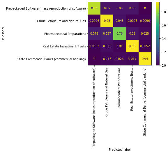
We can see from the above confusion matrix that cosine similarity analysis on 2-to-4 grams embeddings give an accuray of 89% on average. For industries Crude Petroleum and Natural Gas, Real Estate Investment Trusts and State Commercial Banks (commercial banking), the accuracy is above 90%. Pharmaceutical Preparations gives the lowest accuracy at 76%.
Plotting
Plotting on the Cosine Similarity Matrix
We use PCA to automatically perform dimensionality reduction. First, we have a 2-D plot on cosine similarity matrix.
plot_cos = std_func.pca_visualize_2d(cosine_sim, df.loc[:,["name","SIC_desc"]])
Here we have a 3-D plot with the first three dimensions which maximize the most variance.
std_func.pca_visualize_3d(plot_cos)
We can see from the above 3D plot that three industries are clustered well spread, especially state commercial banks. However, prepackaged software industry is closely clustered with the others.
We can look at the explained variance of each dimension the PCA embedding of our cosine similatiry matrix produced below:
plot_cos[0].explained_variance_ratio_
array([0.43705121, 0.21549028, 0.13752174, 0.05257744, 0.03654605,
       0.01467293, 0.00914707, 0.00835553, 0.0072873 , 0.00633825])
The total explained variance of the first three dimensions are:
plot_cos[0].explained_variance_ratio_[0:3].sum()
0.7900632276689792
The first three dimensions explained 79% of the total variance that exists within the data.
Conclusion Reporting
from sklearn.metrics import classification_report
print(classification_report(prediction["y_true"], prediction["y_pred"], target_names=df["SIC_desc"].unique()))
                                                      precision    recall  f1-score   support

Prepackaged Software (mass reproduction of software)       0.88      0.85      0.87        80
                     Crude Petroleum and Natural Gas       0.91      0.93      0.92       208
                         Pharmaceutical Preparations       0.77      0.76      0.77        80
                       Real Estate Investment Trusts       0.94      0.95      0.94       191
         State Commercial Banks (commercial banking)       0.96      0.94      0.95       116

                                            accuracy                           0.91       675
                                           macro avg       0.89      0.89      0.89       675
                                        weighted avg       0.91      0.91      0.91       675
We can see from the above classification_report, we can conclude that cosine similarity analysis on 2-to-4 grams embeddings gives a good result on SIC classfication, specifically on the industries Crude Petroleum and Natural Gas, Real Estate Investment Trusts and State Commercial Banks (commercial banking).