LDA (Latent Dirichlet Allocation)

LDA (Latent Dirichlet Allocation)¶

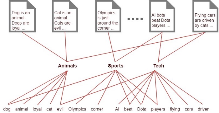
LDA is a generative statistical model that allows sets of observations to be explained by unobserved groups that explain why some parts of the data are similar. For example, if observations are words collected into documents, it posits that each document is a mixture of a small number of topics and that each word’s presence is attributable to one of the document’s topics.

To connect this back to bag-of-words (term frequency), the former approach can be thought of as a simplistic probabilistic model of documents as distributions over words. The bag-of-words vector then represents the best approximation we have for the unnormalized distribution-of-words in each document; but document here is the basic probabilistic unit, each a single sample of its unique distribution.

The crux of the matter, then, is to move from this simple probabilistic model of documents as distributions over words to a more complex one by adding a latent (hidden) intermediate layer of K topics.

From CSCD25, by Ashton Anderson

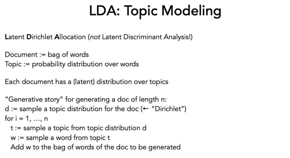
We are explaining documents (companies in our case) by their distribution across topics, which themselves are explained by a distribution of words.

Lets get to the code!¶

First we need to load in the functions and data:

import os
import json
import pandas as pd
import numpy as np
import sys
sys.path.insert(0, '..')
%load_ext autoreload
%autoreload 2
%aimport std_func

df = pd.read_csv("../data/preprocessed.csv")

The LDA decomposition is based off of a tf-idf matrix, which we calculated earlier. As you can see, its quite simple to create a data pipeline that passes our data through the models we want to fit.

from sklearn.decomposition import LatentDirichletAllocation
from sklearn.feature_extraction.text import TfidfTransformer
from sklearn.feature_extraction.text import CountVectorizer
from sklearn.pipeline import Pipeline

pipe = Pipeline([('count', CountVectorizer(
                                           ngram_range = (2,4),
                                           stop_words = 'english', max_features = 600)),
                 ('tfidf', TfidfTransformer()),
                 ('lda', LatentDirichletAllocation(n_components = 8))]).fit(df["coDescription_stopwords"])

Below we have the matrix of our 8 (arbitrarily) chosen topics and their vectors as they lie in our 600 term vector space:

pd.DataFrame(pipe["lda"].components_)

	0	1	2	3	4	5	6	7	8	9	...	590	591	592	593	594	595	596	597	598	599
0	0.125168	0.127951	0.125004	0.125602	0.615018	0.125056	0.896461	0.125125	0.125345	0.125387	...	0.125370	0.125000	1.449715	0.125014	0.125588	0.125701	2.738875	2.698285	1.789115	0.129322
1	0.166339	0.226145	0.125002	0.395087	1.161580	0.472283	3.289610	0.125000	2.644513	0.907269	...	1.806161	0.125000	0.237073	0.166171	1.320508	1.099827	1.970725	1.518579	1.360892	0.952780
2	0.125004	0.125002	0.125000	0.125001	0.125001	0.125001	0.125001	0.125000	0.125001	0.125001	...	0.125001	0.125000	0.125001	0.125004	0.125001	0.125001	0.125001	0.125001	0.125001	0.125001
3	0.125004	0.125002	0.125000	0.125001	0.125001	0.125001	0.125001	0.125000	0.125001	0.125001	...	0.125001	0.125000	0.125001	0.125004	0.125001	0.125001	0.125001	0.125001	0.125001	0.125001
4	0.125003	0.125003	0.125000	0.125001	0.125001	0.125001	0.125016	0.125000	0.125000	0.125001	...	0.125000	0.125000	0.125001	0.125003	0.125001	0.125001	0.125008	0.125003	0.125003	0.125001
5	0.125004	0.125002	0.125000	0.125001	0.125001	0.125001	0.125001	0.125000	0.125001	0.125001	...	0.125001	0.125000	0.125001	0.125004	0.125001	0.125001	0.125001	0.125001	0.125001	0.125001
6	0.872406	0.608333	0.125000	2.214727	1.974145	1.039703	0.813642	3.149322	0.844877	0.318719	...	1.871689	3.161434	1.060711	0.905642	0.915567	0.773850	1.267934	1.116209	1.186985	0.970318
7	2.675404	2.210028	5.457224	0.946824	4.028063	2.511474	3.575978	0.125068	8.097945	3.990221	...	9.400579	0.125002	2.068890	4.641963	4.083440	3.278506	0.808350	15.663433	14.983939	2.630458

8 rows × 600 columns

Below we have the top 5 terms for each topic that we’ve created from our corpus:

		index	variable	value
index
0	2488	0	intellectual property	12.393608
	1248	0	data center	12.071443
	3608	0	professional service	9.372933
	3936	0	report form	8.194866
	3600	0	product service	7.720827
1	817	1	clinical trial	64.325112
	3577	1	product candidate	39.634109
	3465	1	phase clinical	24.440173
	4665	1	united state	22.451268
	3473	1	phase clinical trial	19.094278
2	1330	2	deposit account	0.125010
	850	2	commercial loan	0.125007
	370	2	bank ha	0.125007
	3794	2	ratio le	0.125006
	2674	2	loan commercial	0.125006
3	1331	3	deposit account	0.125010
	851	3	commercial loan	0.125007
	371	3	bank ha	0.125007
	3795	3	ratio le	0.125006
	2675	3	loan commercial	0.125006
4	908	4	common equity	2.421448
	180	4	analysis financial condition result	2.324595
	1420	4	discussion analysis financial condition	2.324502
	1412	4	discussion analysis financial	2.319093
	172	4	analysis financial condition	2.288438
5	1333	5	deposit account	0.125010
	853	5	commercial loan	0.125007
	373	5	bank ha	0.125007
	3797	5	ratio le	0.125006
	2677	5	loan commercial	0.125006
6	2318	6	holding company	40.425221
	382	6	bank holding	30.943883
	390	6	bank holding company	30.053073
	1862	6	federal reserve	24.140566
	1966	6	financial institution	16.974052
7	3807	7	real estate	53.065015
	3047	7	natural gas	32.624739
	943	7	common stock	26.518227
	3231	7	oil natural	20.368836
	3223	7	oil gas	20.205053

Here we transform company reports using the data pipeline we built earlier which gives us a probability of belonging to each of the 8 topics:

lda_df = pd.DataFrame(pipe.transform(df['coDescription']))
lda_df

	0	1	2	3	4	5	6	7
0	0.579219	0.021932	0.021918	0.021918	0.022052	0.021918	0.021935	0.289109
1	0.450110	0.025427	0.025401	0.025401	0.025497	0.025401	0.025417	0.397346
2	0.668230	0.020547	0.020523	0.020523	0.098503	0.020523	0.020542	0.130610
3	0.709804	0.022695	0.022679	0.022679	0.154053	0.022679	0.022693	0.022718
4	0.021047	0.030965	0.019877	0.019877	0.019884	0.019877	0.019885	0.848587
...	...	...	...	...	...	...	...	...
670	0.025365	0.025360	0.025356	0.025356	0.025357	0.025356	0.025375	0.822475
671	0.019291	0.865106	0.019261	0.019261	0.019261	0.019261	0.019266	0.019292
672	0.017807	0.030874	0.017571	0.017571	0.017572	0.017571	0.017585	0.863450
673	0.019964	0.019960	0.019954	0.019954	0.020002	0.019954	0.019976	0.860238
674	0.551868	0.051731	0.051683	0.051683	0.051683	0.051683	0.051735	0.137935

675 rows × 8 columns

Plotting the results¶

Here are the results of running our data through LDA.

You may have noticed that these plots look very… triangular. What these plots visualize are the 8 probability dimensions calculated using LDA and projected to this lower dimensional space.

These embeddings are not exactly helpful in clustering documents together, but they can give us a great view into the latent topics that exist within our corpus.

If we examine the explained variance ratio, we see that the top three dimensions don’t actually explain that much of the variation that exists within our data/companies. This is as expected.

plot[0].explained_variance_ratio_

array([5.43884483e-01, 3.57897683e-01, 7.88731468e-02, 1.85170944e-02,
       8.27592331e-04, 9.11945784e-25, 2.09612832e-32, 7.76262852e-36])

Topic Modelling Introduction

LSA (Latent Semantic Analysis)

Analysis of Textual data from 10K Financial Reports

LDA (Latent Dirichlet Allocation)

Contents

LDA (Latent Dirichlet Allocation)¶

Lets get to the code!¶

Plotting the results¶